机器学习笔记(三)——多元线性回归

1. 模型描述

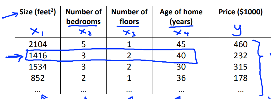
同 单元线性回归 的例子，现在在已知房子 尺寸大小 的情况下，再额外考虑 房间数目、层数、房屋建成年龄 对 房屋价格 的影响。

设假设函数如下：

$h_\theta(x_i)=\theta_0+\theta_1x_{i,1}+\theta_2x_{i,2}+\cdots+\theta_nx_{i,n}$

其中，变量描述如下：

1. $x$ 和 $y$ 代表特征和标签集合
2. $x_i$ 代表第 $i$ 个样本，$y_i$ 代表第 $i$ 个样本的标签，而 $x_{i,j}$ 则代表第 $i$ 个样本的第 $j$ 个特征
3. $m$ 为样本个数，$n$ 为特征种类数量
4. $h_\theta$ 为假设函数
5. $\theta$ 为参数向量，$\theta_i$ 代表假设函数的第 $i$ 个参数

为了方便计算，我们给每个样本的特征加上 $x_{i,0} = 1$ 这个特征，让假设函数变为如下形式：

$\begin{aligned} h_\theta(x_i)&=\theta_0x_{i,0}+\theta_1x_{i,1}+\theta_2x_{i,2}+\cdots+\theta_nx_{i,n}\\ &=\theta^Tx_i \end{aligned}$

2. 代价函数及梯度计算

由上一节所述，则该模型的代价函数可以定义为平方误差函数：

$J(\theta_0,\theta_1,\cdots,\theta_n)=\frac{1}{2m}\sum_{i=1}^{m}(h_\theta(x_i)-y_i)^2$

其梯度变化如下：

$\theta_j=\theta_j-\alpha\frac{1}{m}\sum_{i=1}^m(h_\theta(x_i)-y_i)x_{i,j}$

3. 加快梯度下降的速度

3.1 特征缩放(Feature scaling)

确保特征在相同的值域范围内。假设某个线性回归模型有两个特征，其参数对应 $\theta_1$ 和 $\theta_2$ ，若其特征 $x_1$ 和 $x_2$ 的值域范围不一样，则可能在梯度下降的过程中存在在一个方向上走得快，而另一个方向走得慢，导致其在等高线上蜿蜒前进。

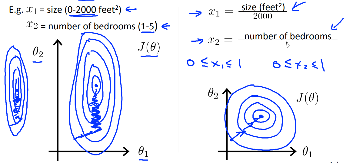
3.2 均值归一化(Mean normalization)

将原来的特征 $x$ 进行均值归一化，使其具有接近 0 的均值，计算公式如下：

$std(x) = \frac{x-mean(x)}{max(x)-min(x)}$

3.3 选择合适的学习速率

对于学习速率 $\alpha$：

• 若过小：则梯度下降缓慢，最终趋于收敛。
• 若过大：则 $J(\theta)$ 可能不是每一次迭代都会下降，而且可能不会收敛。

则需要我们选择合适的学习速率，建议训练的时候绘制出 $J(\theta)$ 在设定学习速率下随迭代次数增加的变化曲线，以找到最合适的学习速率，减少其迭代次数。

学习速率可以按如下序列进行尝试：

$\cdots,0.001,0.003,0.01,0.03,0.1,0.3,1,\cdots$

4. 案列实现

此处，我们创建一个二元线性回归方程 $f(x_1, x_2) = b + a_1x_1+ a_2x_2$，其中 $b=1$， $a = [4, 3]$，然后通过代码去拟合该直线。

代码

import numpy as np


class MyLiner:
    """
    单变量线性函数的拟合类
    使用梯度下降法
    """
    theta = None
    __alpha = 0  # 下降速率
    __eps = 0  # 梯度变化小于此精度则认定不在变化
    __iters = 0  # 迭代次数
    __x = None  # 二维
    __y = None  # 一维
    m = 0  # 样本数量
    n = 0  # 特征个数

    def __h(self, x):
        """
        假设函数 h
        :param x: 传入特征
        :return: 特征 x 在此假设函数下的映射
        """
        return np.dot(x, self.theta)

    def __J(self):
        """
        平均误差函数
        :return:
        """
        return np.mean((self.__h(self.__x) - self.__y) ** 2) / 2

    def __gd(self):
        """
        梯度下降以及更新
        :return: 更新后的 theta
        """
        t_theta = np.zeros(shape=(self.n, 1))  # 创建存放更新后的 theta 列表
        for j in range(self.n):
            xj = np.array([self.__x[:, j]]).transpose()
            t_theta[j][0] = self.theta[j][0] - self.__alpha * np.mean((self.__h(self.__x) - self.__y) * xj)
        return t_theta

    def __init__(self, alpha=0.1, eps=1e-5, iters=10000):
        """
        构造函数
        :param alpha: 学习步长
        :param eps: 精度
        """
        self.__alpha = alpha
        self.__eps = eps
        self.__iters = iters

    def fit(self, x, y):
        """
        进行训练
        :param x: 特征向量
        :param y: 标签
        """
        self.m, self.n = x.shape[0], x.shape[1] + 1
        self.__y = y
        c = np.ones(shape=(self.m, 1))
        self.__x = np.concatenate((c, x), axis=1)  # 将特征的第一维添加1，方便计算

        self.__x, self.__y = self.__x.astype(np.float64), self.__y.astype(np.float64)

        # 随机找一个起点
        self.theta = np.random.randint(10, size=(self.n, 1))

        tj = self.__J()
        for i in range(self.__iters):  # 进行迭代
            self.theta = self.__gd()
            tj = self.__J()
        return tj

    def get_param(self):
        """
        获取拟合最优的参数
        :return: theta
        """
        return self.theta.flatten()

    def predict(self, x):
        """
        预测
        :param x: 要预测的特征
        :return: 预测的结果
        """
        c = np.ones(shape=(x.shape[0], 1))
        x = np.concatenate((c, x), axis=1)  # 将特征的第一维添加1，方便计算
        return self.__h(x).transpose()


def f(x, a, b):
    """
    自定义线性函数
    :param a:特征对应的系数矩阵
    :param b:常数项
    :param x:特征
    """
    return np.dot(x, a.transpose()) + b


# 生成 f(x) = b + a[1] * x[1] + a[2] * x[2] + ... + a[n] * x[n]
a = np.array([[4, 3]])  # 系数
b = 1
x = np.random.randint(10, size=(20, a.shape[1]))

# 处理 x 并生成 y
y = f(x, a, b)

# 构建模型
model = MyLiner(alpha=0.01, iters=10000)
res = model.fit(x, y)
print(res)  # 输出平均误差 J(theta)
print(model.get_param())  # 假设函数的参数 theta 列表

结果输出

7.868549906123757e-09
[1.00039689 3.99994972 2.99996158]